Measure cash flows with CostIncome

This notebook introduces the CostIncome class from CLIMADA, which is used to model the financial cash flows of adaptation or risk-reduction measures over time.

Quickstart

A CostIncome object tracks:

• Initial (one-off) costs — the upfront implementation cost

• Periodic costs — recurring expenses (e.g., maintenance)

• Periodic income — recurring revenues (e.g., insurance savings, avoided losses)

• Growth rates — how costs and incomes evolve over time

• Custom cash flows — arbitrary user-defined flows (layered on top)

from climada.entity.measures.cost_income import CostIncome

ci = CostIncome(
    mkt_price_year=2025,
    init_cost=10_000,  # 10 000 upfront
    periodic_cost=5_000,  # 5 000 / year maintenance
    periodic_income=8_000,  # 8 000 / year in avoided losses
    cost_yearly_growth_rate=0.01,
    income_yearly_growth_rate=0.01,
    freq="Y",  # annual cash flows
)

impl_date = "2022-01-01"
start_date = "2020-01-01"
end_date = "2030-01-01"


display(ci.to_dataframe(impl_date, start_date, end_date))
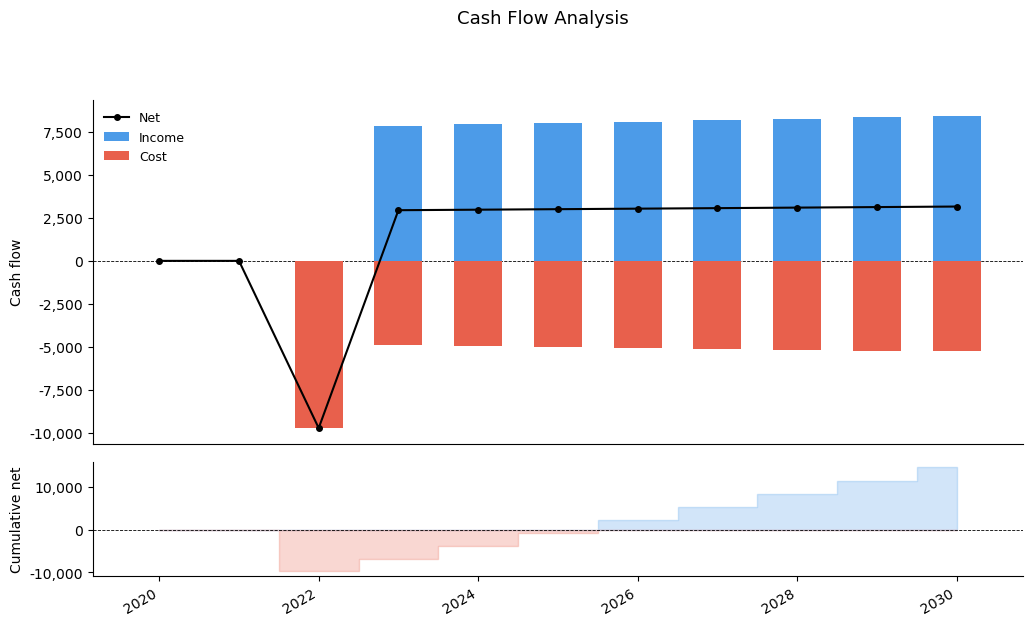
ci.plot_cash_flows(impl_date, start_date, end_date)

	date	net	cost	income
0	2020	0.000000	0.000000	0.000000
1	2021	0.000000	0.000000	0.000000
2	2022	-9705.636889	-9705.636889	0.000000
3	2023	2940.807977	-4901.346629	7842.154606
4	2024	2970.216057	-4950.360095	7920.576152
5	2025	3000.000000	-5000.000000	8000.000000
6	2026	3030.000000	-5050.000000	8080.000000
7	2027	3060.300000	-5100.500000	8160.800000
8	2028	3090.903000	-5151.505000	8242.408000
9	2029	3121.897135	-5203.161892	8325.059028
10	2030	3153.116107	-5255.193511	8408.309618

(<Axes: ylabel='Cash flow'>, <Axes: ylabel='Cumulative net'>)

Defining a CostIncome

The simplest way to create a CostIncome is by passing keyword arguments directly.

Parameter	Meaning
init_cost	One-off implementation cost
periodic_cost	Recurring cost each period
periodic_income	Recurring income each period
mkt_price_year	Reference year for cost/income growth rates
cost_yearly_growth_rate	Growth rate for costs
income_yearly_growth_rate	Growth rate for costs
freq	Period frequency (e.g. 'Y' for yearly, 'M' for monthly, 'Q' for quaterly) see more here)

Note

Sign convention CostIncome stores costs as negative numbers internally.

Note

Financial values in CostIncome are currently unitless (no currency is specified)

from climada.entity.measures.cost_income import CostIncome

ci = CostIncome(
    mkt_price_year=2025,
    init_cost=10_000,  # 10 000 upfront
    periodic_cost=5_000,  # 5 000 / year maintenance
    periodic_income=8_000,  # 8 000 / year in avoided losses
    cost_yearly_growth_rate=0.01,
    income_yearly_growth_rate=0.01,
    freq="Y",  # annual cash flows
)

Calculating cash flows

Three methods are available to calculate cash flows:

Method	Returns
calc_cash_flows(impl_date, start_date, end_date)	Three np.ndarray: net, costs, incomes
calc_total(impl_date, start_date, end_date)	Three scalars: summed net, cost, income
to_dataframe(impl_date, start_date, end_date)	A tidy pd.DataFrame

The impl_date is when the measure is deployed. Cash flows before this date are zero; the initial cost lands on impl_date; periodic flows start the following period.

Note

Dates should follow the standard format “yyyy-mm-dd” or be an integer representing the year.

import pandas as pd

impl_date = "2022-01-01"
start_date = "2020-01-01"
end_date = "2030-01-01"

net, costs, incomes = ci.calc_cash_flows(impl_date, start_date, end_date)
total_net, total_cost, total_income = ci.calc_total(impl_date, start_date, end_date)

print("Period  | Net       | Cost      | Income")
print("-" * 45)
periods = pd.period_range(start=start_date, end=end_date, freq="Y")
for p, n, c, i in zip(periods, net, costs, incomes):
    print(f"{p}  | {n:>9.0f} | {c:>9.0f} | {i:>6.0f}")
print("-" * 45)
print(f"Total net    : {total_net:>10.0f}")
print(f"Total cost   : {total_cost:>10.0f}")
print(f"Total income : {total_income:>10.0f}")
print("-" * 45)

Period  | Net       | Cost      | Income
---------------------------------------------
2020  |         0 |         0 |      0
2021  |         0 |         0 |      0
2022  |     -9706 |     -9706 |      0
2023  |      2941 |     -4901 |   7842
2024  |      2970 |     -4950 |   7921
2025  |      3000 |     -5000 |   8000
2026  |      3030 |     -5050 |   8080
2027  |      3060 |     -5100 |   8161
2028  |      3091 |     -5152 |   8242
2029  |      3122 |     -5203 |   8325
2030  |      3153 |     -5255 |   8408
---------------------------------------------
Total net    :      14662
Total cost   :     -50318
Total income :      64979
---------------------------------------------

ci.to_dataframe(impl_date, start_date, end_date)

	date	net	cost	income
0	2020	0.000000	0.000000	0.000000
1	2021	0.000000	0.000000	0.000000
2	2022	-9705.636889	-9705.636889	0.000000
3	2023	2940.807977	-4901.346629	7842.154606
4	2024	2970.216057	-4950.360095	7920.576152
5	2025	3000.000000	-5000.000000	8000.000000
6	2026	3030.000000	-5050.000000	8080.000000
7	2027	3060.300000	-5100.500000	8160.800000
8	2028	3090.903000	-5151.505000	8242.408000
9	2029	3121.897135	-5203.161892	8325.059028
10	2030	3153.116107	-5255.193511	8408.309618

Visualising cash flows

plot_cash_flows draws a bar chart of the cash flows. The top panel of the plot shows costs, incomes and net values for each period, while the bottom panel shows the cumulated net value.

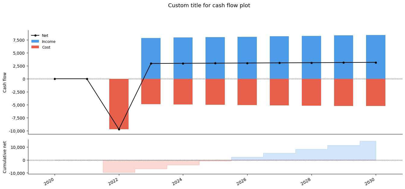
Figure size and title can be customized directly in the method. The method returns a tuple with the two matplotlib axes objects.

ci.plot_cash_flows(
    impl_date,
    start_date,
    end_date,
    figsize=(16, 7),
    title="Custom title for cash flow plot",
)

(<Axes: ylabel='Cash flow'>, <Axes: ylabel='Cumulative net'>)

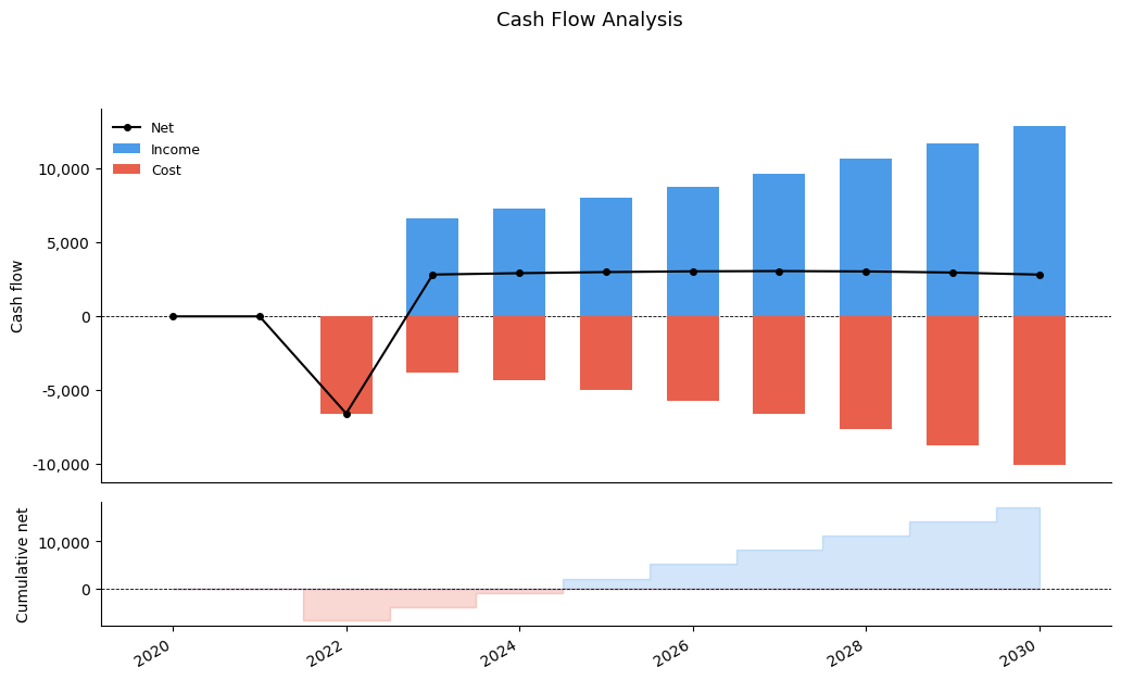
Growth rates

Costs and incomes can grow year-over-year using compound-interest factors anchored to the mkt_price_year attribute.

\[\text{value}(t) = \text{base} \times (1 + r)^{\frac{t - t_0}{365}}\]

Pass cost_yearly_growth_rate and / or income_yearly_growth_rate (as decimals, e.g. 0.02 for 2 %).

ci_growth = CostIncome(
    mkt_price_year=2025,
    init_cost=10_000,
    periodic_cost=5_000,
    periodic_income=8_000,
    cost_yearly_growth_rate=0.15,
    income_yearly_growth_rate=0.10,
    freq="Y",
)

ci_growth.plot_cash_flows(impl_date, start_date, end_date)

(<Axes: ylabel='Cash flow'>, <Axes: ylabel='Cumulative net'>)

# Compare totals with and without growth
no_growth = ci.calc_total(impl_date, start_date, end_date)
with_growth = ci_growth.calc_total(impl_date, start_date, end_date)

labels = ["Net", "Cost", "Income"]
print(f"{'':15s} {'No growth':>12s} {'With growth':>12s}")
for label, ng, wg in zip(labels, no_growth, with_growth):
    print(f"{label:15s} {ng:>12.0f} {wg:>12.0f}")

                   No growth  With growth
Net                    14662        17138
Cost                  -50318       -58474
Income                 64979        75612

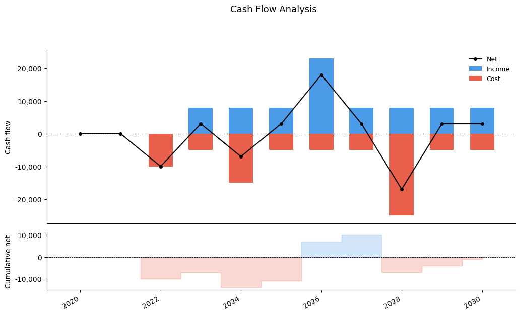
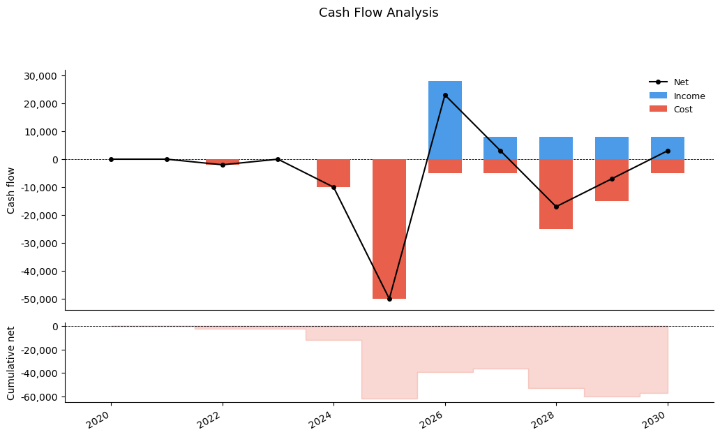
Custom cash flows

For irregular or one-off flows, pass a pd.DataFrame with columns date, cost, and/or income.

These are added on top of any periodic amounts; dates not present in the DataFrame simply contribute zero.

custom_flows = pd.DataFrame(
    {
        "date": ["2024-01-01", "2026-01-01", "2028-01-01"],
        "cost": [10_000, 0, 20_000],  # extra one-off costs
        "income": [0, 15_000, 0],  # extra one-off income
    }
)

ci_custom = CostIncome(
    mkt_price_year=2025,
    init_cost=10_000,
    periodic_cost=5_000,
    periodic_income=8_000,
    custom_cash_flows=custom_flows,
    freq="Y",
)
ci_custom.to_dataframe(impl_date, start_date, end_date)

	date	net	cost	income
0	2020	0.0	0.0	0.0
1	2021	0.0	0.0	0.0
2	2022	-10000.0	-10000.0	0.0
3	2023	3000.0	-5000.0	8000.0
4	2024	-7000.0	-15000.0	8000.0
5	2025	3000.0	-5000.0	8000.0
6	2026	18000.0	-5000.0	23000.0
7	2027	3000.0	-5000.0	8000.0
8	2028	-17000.0	-25000.0	8000.0
9	2029	3000.0	-5000.0	8000.0
10	2030	3000.0	-5000.0	8000.0

ci_custom.plot_cash_flows(impl_date, start_date, end_date)

(<Axes: ylabel='Cash flow'>, <Axes: ylabel='Cumulative net'>)

Sub-annual frequencies

freq accepts any pandas-compatible period aliases string.

Common options:

freq	Meaning
"Y"	Annual
"Q"	Quarterly
"M"	Monthly
"7D"	Every 7 days

Note

The periodic amounts are interpreted as per-period values. A periodic cost of 500 with a monthly frequency (“M”), means a cost of 500 per month. The growth rates however are always considered to be yearly.

Note

The implementation, starting and ending dates are coerced to the period frequency. For instance "2022-01-05" with monthly frequency is considered as "2022-01".

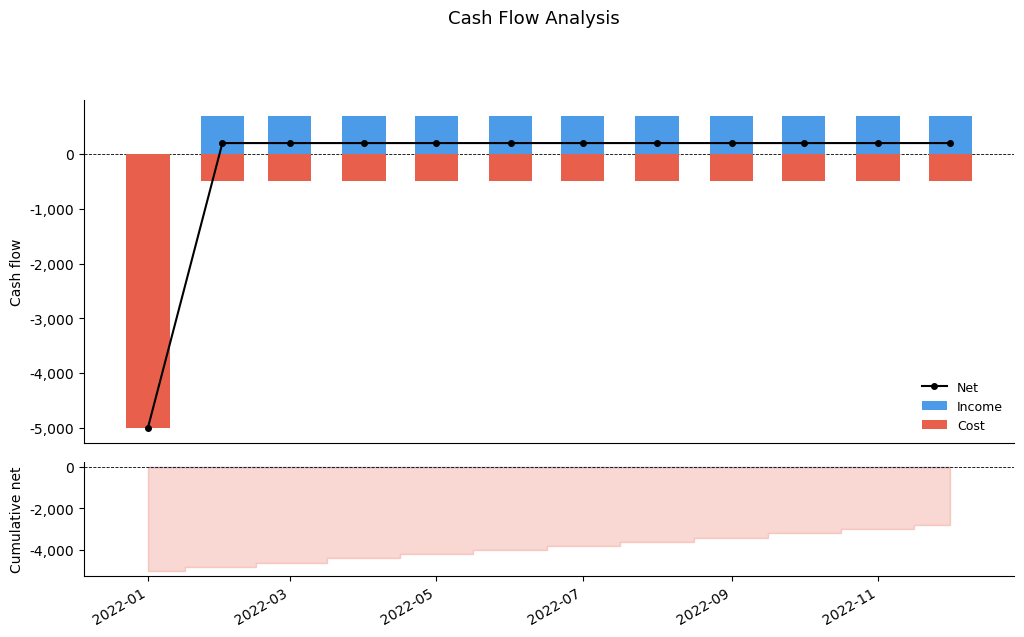
ci_monthly = CostIncome(
    mkt_price_year=2022,
    init_cost=5_000,
    periodic_cost=500,
    periodic_income=700,
    freq="M",
)

df_monthly = ci_monthly.to_dataframe(
    impl_date="2022-01-05",
    start_date="2022-01",
    end_date="2022-12",
)
df_monthly

	date	net	cost	income
0	2022-01	-5000.0	-5000.0	0.0
1	2022-02	200.0	-500.0	700.0
2	2022-03	200.0	-500.0	700.0
3	2022-04	200.0	-500.0	700.0
4	2022-05	200.0	-500.0	700.0
5	2022-06	200.0	-500.0	700.0
6	2022-07	200.0	-500.0	700.0
7	2022-08	200.0	-500.0	700.0
8	2022-09	200.0	-500.0	700.0
9	2022-10	200.0	-500.0	700.0
10	2022-11	200.0	-500.0	700.0
11	2022-12	200.0	-500.0	700.0

ci_monthly.plot_cash_flows(
    "2022-01",
    "2022-01",
    "2022-12",
)

(<Axes: ylabel='Cash flow'>, <Axes: ylabel='Cumulative net'>)

Combining multiple CostIncome objects

CostIncome.comb_cost_income() aggregates a list of CostIncome objects into a single one by summing costs and incomes.

Warning

All objects must share the same mkt_price_year, cost_growth_rate, and income_growth_rate.

Note

custom_cash_flows are merged by summing them together.

import pandas as pd

custom_flows_a = pd.DataFrame(
    {
        "date": ["2024", "2026", "2028"],
        "cost": [10_000, 0, 20_000],  # extra one-off costs
        "income": [0, 15_000, 0],  # extra one-off income
    }
)

custom_flows_b = pd.DataFrame(
    {
        "date": ["2022", "2026", "2029"],
        "cost": [2_000, 0, 10_000],  # extra one-off costs
        "income": [0, 5_000, 0],  # extra one-off income
    }
)

ci_a = CostIncome(
    mkt_price_year=2020,
    init_cost=30_000,
    periodic_cost=2_000,
    periodic_income=4_000,
    custom_cash_flows=custom_flows_a,
    freq="Y",
)

ci_b = CostIncome(
    mkt_price_year=2020,
    init_cost=20_000,
    periodic_cost=3_000,
    periodic_income=4_000,
    custom_cash_flows=custom_flows_b,
    freq="Y",
)

ci_combined = CostIncome.comb_cost_income([ci_a, ci_b])
ci_combined.plot_cash_flows(
    "2025",
    "2020",
    "2030",
)

ci_combined.custom_cash_flows

	cost	income
date
2022-01-01	-2000	0
2023-01-01	0	0
2024-01-01	-10000	0
2025-01-01	0	0
2026-01-01	0	20000
2027-01-01	0	0
2028-01-01	-20000	0
2029-01-01	-10000	0

Loading from dict / YAML

From a Python dictionary

config_dict = {
    "mkt_price_year": 2020,
    "init_cost": 50_000,
    "periodic_cost": 5_000,
    "periodic_income": 8_000,
    "cost_yearly_growth_rate": 0.02,
    "income_yearly_growth_rate": 0.03,
    "freq": "Y",
}

ci_from_dict = CostIncome.from_dict(config_dict)
print(ci_from_dict)

CostIncome(
  mkt_price_year          = 2020
  freq                    = 'Y'
  init_cost               = -50,000.00
  periodic_cost           = -5,000.00
  periodic_income         = 8,000.00
  cost_yearly_growth_rate = 2.00%
  income_yearly_growth_rate = 3.00%
  custom_cash_flows       = None
)

From a YAML file

Create a YAML file structured as follows, then load it with CostIncome.from_yaml(<path to file>).

# measure_cost.yaml
cost_income:
  mkt_price_year: 2020
  init_cost: 50000
  periodic_cost: 5000
  periodic_income: 8000
  cost_yearly_growth_rate: 0.02
  income_yearly_growth_rate: 0.03
  freq: "Y"
  # Optional custom flows:
  # custom_cash_flows:
  #   - date: "2024-01-01"
  #     cost: 10000
  #     income: 0

---

# Inside Notebook or script
ci_from_yaml = CostIncome.from_yaml("measure_cost.yaml")